It is easy to see that AUC can be misleading when used to compare two classifiers if their ROC curves cross. Classifier A may produce a higher AUC than B, while B performs better for a majority of the thresholds with which you may actually use the classifier. And in fact empirical studies have shown that it is indeed very common for ROC curves of common classifiers to cross. There are also deeper reasons why AUC is incoherent and therefore an inappropriate measure (see references below).
In this post however, I'll describe the common scenario of training a classifier on highly imbalanced problems (where the data is such that one class has many more examples than another). We only discuss binary classification in this post, so there are only two classes. The AUC measure, is of course, insensitive to class imbalance, but produces rather misleading results. Consider a problem where we have a large number of negative examples and a small number of positive examples. Further, a large number of negative examples are “easy” -- that is you can get most of them right without much effort. This is a fairly common situation with problems like spam/fraud detection in various domains. In such a situation, a classifier that gets the “easy” negatives right, but offers random predictions for the rest, actually does really well on AUC:
(Example below uses the AUC library in R)
n <- 5000
# For this scenario, we use 80% easy negatives (value 0), and the remaining 20% are evenly balanced between positives and negatives (values 1, and -1).
d <- sample( c(numeric(8), -1, 1), n, replace=TRUE)
# Labels maps all negatives to 0, all positives to 1.
labels <- factor((d > 0) * 1)
# We predict all easy negatives correctly, and random predictions for the rest.
rand_preds <- runif(n) * abs(d)
# All easy negatives correct, better predictions for rest with some noise.
good_preds <- d*.1 + rand_preds
# All easy negatives correct. Better, less noisy predictions for the rest.
better_preds <- d*.3 + rand_preds
|
Now examine the AUC-ROC for these predictors:
> auc(roc(rand_preds, labels))
[1] 0.9430441
> auc(roc(good_preds, labels))
[1] 0.9628872
> auc(roc(better_preds, labels))
[1] 0.9896737
|
A couple of observations:
- While technically ‘rand_preds’ only gets the easy examples right, and is no better than random on the ones that matter, it produces a very high AUC of 0.94.
- Because of the large number of true negatives, the differences between the random, good, and better predictors are very small (of the order of 2%-3% change in AUC).
If you increase the imbalance to be 98% easy negatives, and 2% hard positives and negatives, the AUC differences are even smaller:
# 98% easy negatives:
d <- sample( c(numeric(98), -1, 1), n, replace=TRUE)
> auc(roc(rand_preds, labels))
[1] 0.995519
> auc(roc(good_preds, labels))
[1] 0.9974802
> auc(roc(better_preds, labels))
[1] 0.9996038
|
If your problem-specific metric is something like Precision@Recall=80%, these classifiers behave *very* differently:
#Plot Precision-Recall curves (using the ROCR library)
plot(performance(prediction(better_preds, labels), "prec", "rec"), col='green')
plot(performance(prediction(good_preds, labels), "prec", "rec"), col='blue', add=TRUE)
plot(performance(prediction(rand_preds, labels), "prec", "rec"), col='red', add=TRUE)
|
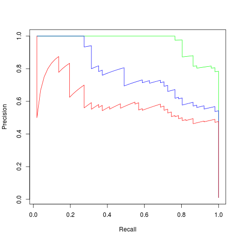 |
| Precision-Recall Curves for the three classifiers |
Precision@Recall=80% for the ‘random’ predictor is ~0.5 (as expected), for the ‘good’ predictor is ~0.65 and the ‘better’ predictor is ~0.9. These differences are huge compared to the AUC numbers which only differ in the third significant digit.
Of course, everybody would recommend using a problem-specific measure ahead of a more generic measure like AUC, the point of this post is to argue that even if you're only using AUC for a quick-and-dirty comparison you shouldn't look at a high value in imbalanced problems and be impressed with the performance.
Jesse Davis and Mark Goadrich. The relationship between Precision-Recall and ROC curves. ICML 2006
D.J. Hand, C. Anagnostopoulos, When is the area under the receiver operating characteristic curve an appropriate measure of classifier performance? Pattern Recognition Letters, Volume 34, Issue 5, 1 April 2013, Pages 492–495
David J. Hand, Measuring classifier performance: a coherent alternative to the area under the ROC curve. Machine Learning October 2009, Volume 77, Issue 1, pp 103-123
This comment has been removed by a blog administrator.
ReplyDelete