UDF Centric Workflows

A recent PVLDB paper titled "An Architecture for Compiling UDF-Centric Workflows" describes some pretty exciting advances in the state of the art for data analysis. Using a system called Tupleware, the authors of the paper show that for datasets that fit into the memory of a small cluster, it is possible to extract far more performance from the hardware than is commonly provided on platforms like Spark. For instance, on a K-Means task, Tupleware was faster than Spark by 5X on a single node, and by nearly 100X on a 10-node cluster. For small datasets, that probably means a 1000x (3 orders of magnitude) improvement over Hadoop.

The dramatic performance improvement come from leveraging several known techniques from the literature on main-memory database systems and compilers. Tupleware relies on combining both high-level optimizations common in relational optimizers (projection and selection pushdown, join order optimization) with optimizations considered by recent main-memory systems like pipelining operators vs. vectorized simple operators. Several techniques and heuristics are described in the paper that produce this combined performance improvement.

Tupleware generates and compiles a program for each workflow, and leaning on the LLVM compiler framework lets it use many techniques like inlining UDFs, SIMD vectorization, generated implementations for context variables, etc. In the distributed setting, Tupleware communicates at the level of blocks of bytes while Spark uses fairly expensive Java serialization that consumes a fair fraction of the runtime for distributed execution. Tupleware does not describe any support for fault-tolerance, but with the huge performance improvement over Spark for many applications, simply restarting the job may be reasonable until we get to a certain job size.

Many researchers have pointed out that the fault-tolerance trade-offs that are right for analysis of large datasets (hundreds of terabytes) are not the same as the ones for smaller datasets (few terabytes). Glad to see data management research that's highlighting this well beyond the "X is faster than Hadoop for T".

Insurance and Self-Driving Cars

Metromile (a car insurance company that's pioneering a pay-as-you-go model) recently produced an analysis of what their monthly insurance rates would be for a self-driving car based on the accident stats that Google released. Check out the expected savings on a variety of models:

No surprise that insurance companies like self-driving cars -- for the kinds of applications we've seen these cars used for, they are much safer than the typical (distracted) American driver. This is one of those world-changing technologies I'm eagerly looking forward to!

Google Could Bigtable : NoSQLaaS

I'm very excited that Google announced Cloud Bigtable. You get a managed instance of Bigtable with an open-source API (there's an HBase client) at a great price! Bigtable's HBase APIs are fairly simple and easy to use, and we seem to have mapped nearly all of the features in the client to Bigtable.

Combined with Google Cloud Dataflow, which lets you write Flume jobs over your data for analytics, I think Google's Cloud Platform is very compelling for data intensive applications. I'm a huge fan of Flume, and am absolutely convinced it provides a huge boost to developer productivity compared to writing direct mapreduces. I think the platform finally has all the pieces needed for big data applications far quicker than rolling-your-own Hadoop+Mapreduce+HBase+Hive/Pig/Scalding stack in the cloud. I'm excited to see how developers will use this platform.

On the dangers of AUC

In most applied ML projects I've been involved in people rarely ever use AUC (the Area Under the ROC Curve) as a performance measure for a classifier. However, it is very commonly reported  in many academic papers. On the surface, the AUC has several nice properties: it is threshold free; so you can compute AUC without having to pick an classification threshold, it is insensitive to changes in the ratio of positive to negative examples in the evaluation set, and it has the nice property that a random classifier has an AUC of 0.5.  

It is easy to see that AUC can be misleading when used to compare two classifiers if their ROC curves cross. Classifier A may produce a higher AUC than B, while B performs better for a majority of the thresholds with which you may actually use the classifier. And in fact empirical studies have shown that it is indeed very common for ROC curves of common classifiers to cross. There are also deeper reasons why AUC is incoherent and therefore an inappropriate measure (see references below).

In this post however, I'll describe the common scenario of training a classifier on highly imbalanced problems (where the data is such that one class has many more examples than another). We only discuss binary classification in this post, so there are only two classes. The AUC measure, is of course, insensitive to class imbalance, but produces rather misleading results. Consider a problem where we have a large number of negative examples and a small number of positive examples. Further, a large number of negative examples are “easy” -- that is you can get most of them right without much effort. This is a fairly common situation with problems like spam/fraud detection in various domains. In such a situation, a classifier that gets the “easy” negatives right, but offers random predictions for the rest, actually does really well on AUC:

(Example below uses the AUC  library in R)

n <- 5000 # For this scenario, we use 80% easy negatives (value 0), and the remaining 20% are evenly balanced between positives and negatives (values 1, and -1). d <- sample( c(numeric(8), -1, 1), n, replace=TRUE) # Labels maps all negatives to 0, all positives to 1. labels <- factor((d > 0) * 1) # We predict all easy negatives correctly, and random predictions for the rest. rand_preds <- runif(n) * abs(d) # All easy negatives correct, better predictions for rest with some noise. good_preds <- d*.1 + rand_preds # All easy negatives correct. Better, less noisy predictions for the rest. better_preds <- d*.3 + rand_preds

Now examine the AUC-ROC for these predictors:

> auc(roc(rand_preds, labels)) [1] 0.9430441 > auc(roc(good_preds, labels)) [1] 0.9628872 > auc(roc(better_preds, labels)) [1] 0.9896737

A couple of observations:

1. While technically ‘rand_preds’ only gets the easy examples right, and is no better than random on the ones that matter, it produces a very high AUC of 0.94.
2. Because of the large number of true negatives, the differences between the random, good, and better predictors are very small (of the order of 2%-3% change in AUC).

If you increase the imbalance to be 98% easy negatives, and 2% hard positives and negatives, the AUC differences are even smaller:

# 98% easy negatives: d <- sample( c(numeric(98), -1, 1), n, replace=TRUE) > auc(roc(rand_preds, labels)) [1] 0.995519 > auc(roc(good_preds, labels)) [1] 0.9974802 > auc(roc(better_preds, labels)) [1] 0.9996038

If your problem-specific metric is something like Precision@Recall=80%, these classifiers behave *very* differently:

#Plot Precision-Recall curves (using the ROCR library) plot(performance(prediction(better_preds, labels), "prec", "rec"), col='green') plot(performance(prediction(good_preds, labels), "prec", "rec"), col='blue', add=TRUE) plot(performance(prediction(rand_preds, labels), "prec", "rec"), col='red', add=TRUE)

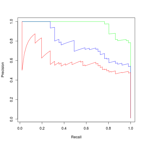Precision-Recall Curves for the three classifiers

Precision@Recall=80% for the ‘random’ predictor is ~0.5 (as expected), for the ‘good’ predictor is ~0.65 and the ‘better’ predictor is ~0.9. These differences are huge compared to the AUC numbers which only differ in the third significant digit.

Of course, everybody would recommend using a problem-specific measure ahead of a more generic measure like AUC, the point of this post is to argue that even if you're only using AUC for a quick-and-dirty comparison you shouldn't look at a high value in imbalanced problems and be impressed with the performance.

Some interesting references:
Jesse Davis and Mark Goadrich. The relationship between Precision-Recall and ROC curves. ICML 2006

D.J. Hand, C. Anagnostopoulos, When is the area under the receiver operating characteristic curve an appropriate measure of classifier performance? Pattern Recognition Letters, Volume 34, Issue 5, 1 April 2013, Pages 492–495

David J. Hand, Measuring classifier performance: a coherent alternative to the area under the ROC curve. Machine Learning October 2009, Volume 77, Issue 1, pp 103-123

WSDM 2015

I recently got back from WSDM which ended up being a very interesting conference with some great talks.

Keynotes

I enjoyed all three keynotes. Mike Franklin's talk focused on AMPLab's research progress and the steady stream of artifacts they've assembled into the Berkeley Data Analytics Stack (BDAS -- pronounced "bad-ass" :)). In addition to Spark, the stack now includes SparkSQL, GraphX, MLLib, Spark Streaming, and Velox. All of these projects pose interesting systems questions and have made a lot of progress on the kinds of tooling that will come in handy for large scale data analysis beyond SQL queries.

Lada Adamic's talk was a fun visual tour through lots of interesting analyses of Facebook data that her team has been running. In particular, she's been using the data to understand what makes a particular piece of content rapidly gain a lot of popularity (or go "viral"). "Sharing" behavior is unique to social networks -- traditional web properties have spent lots of energy understanding what makes people click. The "share" action is a completely different beast to study. Lada reported that they have had some success predicting if a piece of content, once it reaches K users, if it will get to 2K. The prediction accuracy improves as we get to larger K. Unfortunately, she reported that the features that predict virality mostly have to do with the speed at which it is spreading, so we don't yet have a handle on how best to craft viral content

Thorsten Joachims had a technical keynote that followed the arc of his previous work on learning to rank in the context of search. He talked about careful design of interventions in interactive processes to elicit information that can be suitably leveraged by a machine learning algorithm to improve ranking. Lots of examples with evidence from experiments he ran with the arxiv search prototype that have since been reproduced by Yahoo, Baidu, etc.

Research Talks

Here's a subset of research talks that I thought were fun and interesting:

• Delayed-Dynamic-Selective (DDS) Prediction for Reducing Extreme Tail Latency in Web Search: a nice example of exploiting the nature of search servers to go beyond the standard techniques described in the Tail at Scale, which I talked about recently. The paper was the runner-up best paper award.
• Robust Tree-based Causal Inference for Complex Ad Effectiveness Analysis: applying causal inference techniques to ad-campaign data.
• FLAME: A Probabilistic Model Combining Aspect Based Opinion Mining and Collaborative Filtering: ideas on how to better model aspects of a user-rating when there's some text in addition to a numeric rating. Amazon product reviews being an obvious example.
• Just in Time Recommendations – Modeling the Dynamics of Boredom in Activity Streams: modeling repeat consumption of music and figuring out when a user wants to listen to more music of the same kind (same artist, same album) vs. when the user has gotten bored, and wants to move on to something else.
• User Modeling for a Personal Assistant: Srikant's talk on the user-modeling that goes into Google Now. Fun insights into the practical problems that were solved to build Google Now cards.
• Inverting a Steady-State: the best paper award winner from our group at Google.

The Tail at Scale

Another blog post recommending a paper to read ....

One of the challenges of building large systems on shared infrastructure like AWS and the Google Cloud is that you may have to think harder about dealing with variations in response time than you might if you were designing for dedicated hardware (like a traditional data warehouse).  This is obviously critical when you're building latency-critical services that power interactive experiences (websites, mobile apps, video/audio streaming services, etc.). Depending on the operating point, you're likely to see this effect even with batch processing systems like Map-Reduce and large scale machine learning systems.

A CACM article from Jeff Dean and Luiz Andre Barosso -- The Tail at Scale contains many valuable lessons on how to engineer systems to be robust to tail latencies. Some of the interesting ideas from the paper are to use:

1. Hedged requests: The client sends a request to one replica, and after a short delay, sends a second request to another replica. As soon as one response is received, the other request is cancelled.
2. Tied requests: The client sends a request to two replicas (also with a short delay) making sure the requests have metadata so that they know about each other. As soon as one replica starts processing a request, it sends a cancellation message to the other replica (this keeps the client out of the loop for the cancel-logic). Proper implementations of hedged requests and tied requests can significantly improve the 99th percentile latency with a negligible (2% - 3%) increase in the number of requests sent.
3. Oversharding/Micro-Partitions: The portion of data to be served is divided into many more shards than there are machines to serve them. Each server is assigned several shards to manage. This way, load balancing can be managed in a fairly fine-grained manner by moving a small number of shards at a time from one server to another. This allows us better control in managing the variability in load across machines. Systems like Bigtable (and open-source implementations like HBase), for instance, have servers that each manage dozens of shards.

There are lots of other ideas and interesting discussions in the paper. I strongly recommend it!